Introducción

En documentos previos de esta serie hemos abordado cómo evaluar la validez de una prueba diagnóstica. También hemos revisado cómo medir su precisión o fiabilidad. Hasta ahora hemos mostrado los métodos de medición de la precisión para datos discretos nominales (índice kappa) y ordinales (índice kappa ponderado). Ahora abordaremos los métodos correspondientes a datos continuos: la desviación estándar intrasujetos, el coeficiente de correlación intraclase y el método de Bland y Altman.

Variables continuas

Desviación estándar intrasujetos

Cuando el resultado de una prueba se mide en una escala continua, podemos estimar el error de medición calculando la variabilidad existente entre medidas repetidas en los mismos sujetos. El parámetro que mejor refleja dicha variabilidad es la desviación estándar intrasujetos (excluyendo la observada entre sujetos). Para calcularlo necesitamos una serie de sujetos a los que se les realicen al menos dos mediciones. En la tabla 1 se presentan los resultados de dos mediciones repetidas de bilirrubina transcutánea en recién nacidos ictéricos¹. La desviación estándar intrasujetos puede calcularse fácilmente usando un programa que realice análisis de la varianza (ANOVA). El ANOVA descompone la variación que hay entre el conjunto de mediciones (estimada a través de la diferencia de cada valor respecto la media global al cuadrado) en varios componentes: la variación entre las mediciones de los diferentes sujetos (entre las filas de la tabla 1) y la variación residual, que en una ANOVA de un factor corresponde a la variación entre las mediciones de cada sujeto (entre las columnas de la tabla 1).

Tabla 1. Resultados de dos mediciones repetidas de bilirrubina transcutánea (Jaundice-Meter 101, Minolta Air Shields), en la cara anterior del tórax en 20 recién nacidos ictéricos. Datos extraídos de un estudio más amplio³. Mostrar/ocultar

En la tabla 2 podemos ver el ANOVA para los datos de la tabla 1. El parámetro denominado cuadrados medios de los residuos (CMr) es la varianza residual o intrasujetos (que depende de las diferencias entre las mediciones repetidas de cada sujeto). Si realizamos la raíz cuadrada de CMr obtendremos la desviación estándar intrasujetos (s_i). La s_i puede calcularse igualmente a partir del ANOVA para estudios con más de dos mediciones por sujeto.

Tabla 2. Análisis de la varianza de una vía de los datos de la tabla 1. Mostrar/ocultar

Utilizando la s_i podemos cuantificar el margen de error de nuestras mediciones. Así, podemos estimar que la diferencia entre una medición determinada y el verdadero valor no será mayor de 1,96 veces la s_i en el 95% de las observaciones (asumiendo que siguen una distribución normal, el 95% de las determinaciones caerán en el intervalo entre el valor verdadero más menos 1,96 veces la desviación estándar). También nos permite estimar que la diferencia entre dos mediciones repetidas en un mismo sujeto no superará 2,77 veces la s_i en el 95% de las observaciones^2,3. Para nuestro ejemplo, la s_i es 0,54 (raíz cuadrada de 0,3), por lo que la diferencia estimada respecto al valor verdadero será menor de 1,05 (1,96 × 0,54) y la diferencia entre dos mediciones será menor de 1,49 (2,77 × 0,54).

Coeficiente de correlación intraclase

Si solo se realizan dos mediciones por sujeto, la forma más intuitiva de compararlas es representar las parejas de mediciones en un diagrama de puntos, examinando si existe relación lineal entre ambas y calcular su coeficiente de correlación. En la figura 1 se presenta el diagrama de puntos de los datos de la tabla 1. El coeficiente de correlación de Pearson (r) para estos datos es 0,97 (cuanto más se aproxima a 1, mejor es la correlación).

Figura 1. Diagrama de puntos y correlación lineal de los datos de la tabla 1. Mostrar/ocultar

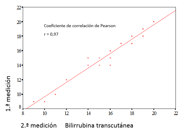
Sin embargo, la existencia de una fuerte relación lineal con un alto coeficiente de correlación no indica que haya una buena concordancia entre las mediciones, solamente que los puntos del diagrama se ajustan a una recta. El coeficiente de correlación depende en gran manera de la variabilidad entre sujetos, por ello, varía mucho en función de las características de la muestra donde se estima, afectándole especialmente la presencia de valores extremos. Si una de las mediciones es sistemáticamente mayor que otra, el coeficiente de correlación será muy alto, a pesar de que las mediciones nunca concuerden. Estos problemas son evitados utilizando el coeficiente de correlación intraclase.

El coeficiente de correlación intraclase (CCI) estima la concordancia entre dos o más medidas repetidas. El cálculo del CCI se basa en un modelo de ANOVA con medidas repetidas, aplicándose distintas fórmulas en función del diseño y los objetivos del estudio⁴. El escenario más simple es aquel en el que estimamos la variabilidad de las medidas, sin tener en cuenta la variabilidad aportada por los distintos observadores (diseño de una vía con factor aleatorio). Considerando este diseño, y utilizando los resultados del ANOVA, podemos calcular el CCI con la siguiente fórmula:

$$CCI=\frac{CMp-CMr}{CMp+(k-1)CMr},$$

donde k es el número de observaciones por sujeto, CMp son los cuadrados medios entre pacientes (que depende de las diferencias de las mediciones entre sujetos) y CMr los cuadrados medios de los residuos (que depende de las diferencias entre las mediciones repetidas de cada sujeto).

Con los datos del ANOVA de la tabla 2 el CCI será:

$$CCI=\frac{19,55-0,30}{19,55+(2-1)0,30}= 0,96.$$

En nuestro ejemplo, apenas hay diferencias entre el CCI y el coeficiente de correlación de Pearson (r). Si el CCI fuera mucho menor que r, habría que pensar que existe un cambio sistemático entre una medida y otra, lo que podría estar causado por un efecto de aprendizaje. En este caso, las mediciones no se habrían realizado en las mismas circunstancias, por lo que no se darían las condiciones para realizar un estudio de fiabilidad⁵.

Método de Bland y Altman

Un método alternativo para analizar la concordancia entre dos observaciones repetidas que se miden en una escala continua es el método gráfico descrito por Bland y Altman⁶. Consiste en representar en un diagrama de puntos la diferencia entre los pares de mediciones contra su media (figura 2). Los puntos tienden a agruparse alrededor del cero para las diferencias entre las dos mediciones, de forma que cuanto mayor sea el grado de dispersión alrededor del cero, peor será el acuerdo entre los dos métodos. Una forma de valorarlo sería dibujar las líneas horizontales en el nivel de diferencia máxima que puede ser tolerable desde el punto de vista clínico y ver si los puntos, o la mayoría de ellos, se agrupan entre estas dos líneas horizontales. De forma alternativa, se puede estimar la desviación estándar de las diferencias y los intervalos entre los que cabe esperar que se encuentre el 95% de ellas.

Figura 2. Método de Bland y Altman con los datos de la tabla 1. Mostrar/ocultar

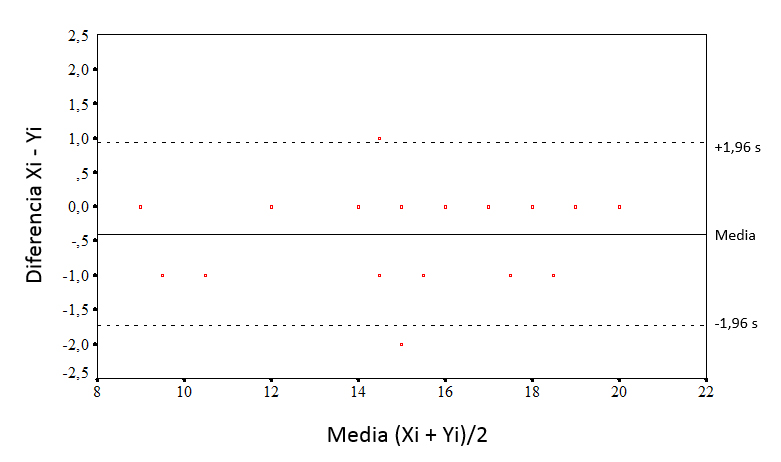
Este método también permite examinar la magnitud de las diferencias y su relación con la magnitud de la medición. Cuando la variabilidad en las medidas no es constante, sino que cambia al aumentar o disminuir la magnitud de la medida, el cálculo se complica⁷. Si existe correlación significativa entre las diferencias y las medias, la variabilidad no será constante (puede haber un acuerdo aceptable en determinado intervalo de valores, pero no en otros). En ese caso, puede intentarse realizar transformaciones logarítmicas de los datos o analizar la variabilidad por separado para varios intervalos de valores, aunque siempre tendremos que cuestionarnos la validez de la medición en ese intervalo.

Bibliografía

1. Ochoa Sangrador C, Marugán Isabel VM, Tesoro González R, García Rivera MT, Hernández Calvo MT. Evaluación de un instrumento de medición de la bilirrubina transcutánea. An Esp Pediatr. 2000;52:561-8.
2. Bland JM, Altman DG. Measurement error. BMJ. 1996;312:1654.
3. Altman DG, Bland JM. Comparing several groups using analysis of variance. BMJ. 1996;312:1472.
4. Fleiss JL. The design and analysis of clinical experiments. Nueva York: John Wiley & Sons 1986. p. 1-32.
5. Bland JM, Altman DG. Measurement error and correlation coefficients. BMJ. 1996;313:41-2.
6. Bland JM, Altman DG. Statistical methods for assessing agreement between two methods of clinical measurement. Lancet. 1986;1:307-10.
7. Bland JM, Altman DG. Measurement error proportional to the mean. BMJ. 1996;313:106.

Introduction

In previous articles in this series, we have addressed how to assess the validity of a diagnostic test. We have also reviewed how to assess its accuracy or reliability. To date, we have discussed the methods used to measure the accuracy of discrete data, nominal (kappa statistic) and ordinal (weighted kappa statistic). In this article, we will broach the methods that apply to continuous data: the within-subject standard deviation, the intraclass correlation coefficient and the Bland and Altman method.

Continuous variables

Within-subject standard deviation

When the result of a test is measured on a continuous scale, we can estimate the measurement error by calculating the variability that exists between repeated measurements in the same subjects. The parameter that best reflects such variability is the within-subject standard deviation (excluding the variability observed between subjects). To calculate it, we need a set of subjects to undergo at least two measurements each. Table 1 presents the results of performing two repeated transcutaneous bilirubin measurements in newborns with jaundice.¹ The within-subject standard deviation can be calculated easily using software that performs analysis of variance (ANOVA). ANOVA breaks down the variation present in the set of measurements (estimated based on the squared differences of each value and the mean of all subjects) into several components: the variation in measurements taken in different subjects (between rows in Table 1) and the variation in the residuals, which in one-way ANOVA corresponds to the variation in the measurements taken in each subject (between columns in Table 1).

Table 1. Results of two repeated transcutaneous bilirubin measurements (Jaundice-Meter 101, Minolta Air Shields) in the anterior surface of the thorax in 20 newborns with jaundice. Data retrieved from a larger study.³ Show/hide

Table 2 shows the ANOVA for the data in Table 1. The parameter called mean square of the residuals (MSr) is the residual or within-subject variance (which depends on the differences between repeated measures in each subject). If we take the square root of the MSr, we obtain the within-subject standard deviation (s_w). The s_w can also be calculated using the results of ANOVA in designs with more than two measurements per subject.

Table 2. One-way analysis of variance for the data in Table 1. Show/hide

We can use the s_w to quantify the margin of error in our measurements. Thus, we can estimate that the difference between a specific measurement and the true value will not be greater than 1.96 times the s_w in 95% of observations (assuming that the data follow a normal distribution, 95% of the measurements will be contained in the interval formed by the actual value plus and minus 1.96 times the standard deviation). It also allows us to estimate that the difference between two measurements for the same subject will not exceed 2.77 times the s_w in 95% of observations.^2,3 In our example, the s_w is 0.54 (square root of 0.3), so the estimated difference from the true value would be of less than 1.05 (1.96 × 0.54) and the difference between two measurements would be of less than 1.49 (2.77 × 0.54).

Intraclass correlation coefficient

If only two measurements are taken per subject, the most intuitive way to compare them is to plot measurement pairs in a scatter diagram, assess whether there is a linear association between them, and calculate the corresponding correlation coefficient. Figure 1 shows the scatter diagram for the data in Table 1. The Pearson correlation coefficient (r) for these data is 0.97 (the closer r is to 1, the stronger the correlation).

Figure 1. Scatter plot and linear correlation for the data in Table 1. Show/hide

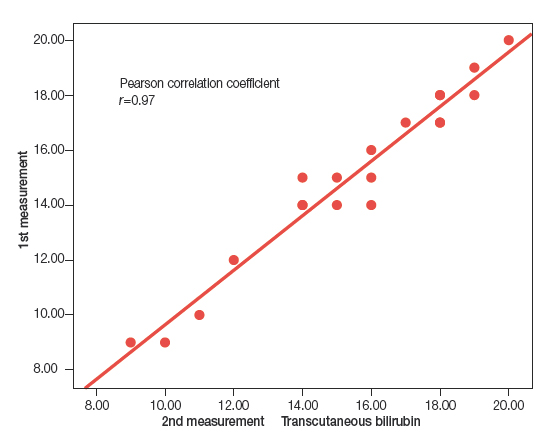
However, the presence of a strong linear association with a high correlation coefficient does not prove a strong agreement between the measurements, but only that the points in the plot fit a straight line well. The correlation coefficient is largely dependent on inter-subject variability and thus changes substantially based on the characteristics of the sample for which it is calculated, and is especially sensitive to the presence of extreme values. If one of the measurements is systematically greater than the other, the correlation coefficient will be very high, despite the fact that the measurements never agree. These pitfalls can be avoiding by using the intraclass correlation coefficient.

The intraclass correlation coefficient (ICC) estimates the agreement between two or more repeated measurements. The calculation of the ICC is based on a repeated measures ANOVA model, applying different formulas based on the design and objectives of the study.⁴ In the simplest scenario, we would estimate the variability of the measurements without taking into account the variability contributed by different raters (one-way random effects model). Choosing this model, and using the results of ANOVA, we can calculate the ICC with the following formula:

$$CCI=\frac{CMp-CMr}{CMp+(k-1)CMr},$$

where k stands for the number of observations per subject, MSp for the mean square between patients (which depends on the differences in measurements between subjects) and MSr for the mean square of the residuals (which depends on the differences between repeated measurements in each subject).

Using the data of the ANOVA in Table 2, the ICC will be:

$$CCI=\frac{19,55-0,30}{19,55+(2-1)0,30}= 0,96.$$

In our example, there is hardly any difference between the ICC and the Pearson correlation coefficient (r). If the ICC were much smaller than r, one would assume that there is a systematic change between one measurement and the other, which may result from a learning effect. In this case, the measurements would not have been made under the same circumstances, so the conditions required for performing a reliability analysis would not be met.⁵

Bland and Altman method

An alternative approach to analysing the agreement between two repeated observations measured on a continuous scale is the graphical method described by Bland and Altman.⁶ It consists of plotting the difference of each pair of measurements against the mean of the two measurements (Figure 2). The points tend to cluster around zero in the axis representing the difference between paired measurements, and the greater the dispersion around zero, the lesser the agreement between the two measurement methods. One possible way to assess agreement is to draw horizontal lines at the level of the maximum difference that would be acceptable from a clinical standpoint, and check whether the points, or most of the points, are grouped between these two horizontal lines. An alternative approach is to estimate the standard deviation of the differences and the interval in which we would expect to find 95% of them.

Figure 2. Bland and Altman method applied to the data in Table 1. Show/hide

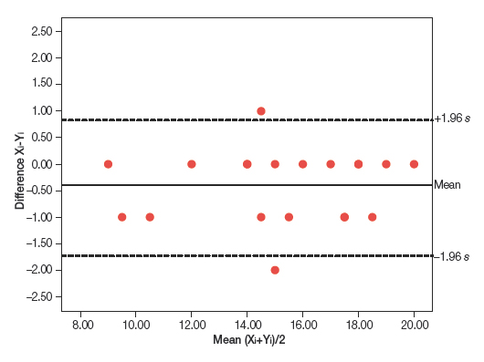
This method can also be used to assess the magnitude of the differences and their association with the magnitude of the measurement. When the variability in the measurements is not constant, but changes as the magnitude of the measurement increases or decreases, the calculation becomes complicated.⁷ If there is a significant correlation between the differences and the means, the variability will not be constant (there may be an acceptable agreement in a specific value interval, but not in others). In this case, a logarithmic transformation of the data can be attempted, or else the variability can be analysed separately for various data intervals, although we should always hold reservations about the validity of measurements in these intervals.

References

1. Ochoa Sangrador C, Marugán Isabel VM, Tesoro González R, García Rivera MT, Hernández Calvo MT. Evaluación de un instrumento de medición de la bilirrubina transcutánea. An Esp Pediatr. 2000;52:561-8.
2. Bland JM, Altman DG. Measurement error. BMJ. 1996;312:1654.
3. Altman DG, Bland JM. Comparing several groups using analysis of variance. BMJ. 1996;312:1472.
4. Fleiss JL. The design and analysis of clinical experiments. New York: John Wiley & Sons 1986. p. 1-32.
5. Bland JM, Altman DG. Measurement error and correlation coefficients. BMJ. 1996;313:41-2.
6. Bland JM, Altman DG. Statistical methods for assessing agreement between two methods of clinical measurement. Lancet. 1986;1:307-10.
7. Bland JM, Altman DG. Measurement error proportional to the mean. BMJ. 1996;313:106.

Cómo citar este artículo

Ochoa Sangrador C, Molina Arias M. Evaluación de la precisión de las pruebas diagnósticas (2). Variables continuas. Evid Pediatr. 2017;13:45.